Where it started
People have compared planetary motion with musical intervals for a long time. Kepler did it in 1619, in the same book that set out his third law of planetary motion.
Sound and visual studies of motion, vibration and pattern across scales.
Musical Universe uses the physics of music to explore motion and repeating patterns across scales. Sound becomes a way to examine relationships that are too slow, too fast or too distant to experience directly. The Uranus and Neptune recording below is one study within that wider inquiry.
Recorded demonstration: orbital motion translated into synthesized sound, with a visual explanation alongside.
Listen for the slow pulse as the sound swells and fades. The pitches stay steady; parts of the two synthesized sounds drift into and out of alignment, like the pulse you listen for while tuning two guitar strings.
Headphones or speakers that carry low tones make the comparison easier to hear. Use a comfortable, steady volume.
The instrument takes orbital rates from a model and shifts them together into a range we can hear, preserving the relationship between them.
The recording compares the original relationship with an exact octave: one tone vibrating twice as fast as the other. Compare the slow pulse with the steadier sound of the adjusted version.
The screen follows the listening comparison, linking the model, the generated tones and their moving waves. This page shows a recording of the locally run instrument.
Still preview · recording to be added
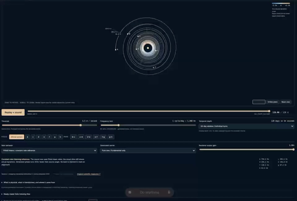
TRAPPIST-1 in a time-history view. The vertical axis represents elapsed model time; the horizontal plane shows the modeled orbital positions.
People have compared planetary motion with musical intervals for a long time. Kepler did it in 1619, in the same book that set out his third law of planetary motion.
Music gives us a familiar way into repetition, proportion and resonance. A string's harmonics and the linked orbital cycles of a system such as TRAPPIST-1 offer concrete relationships to compare across scales. Each system has its own physics; choosing how to turn its data into sound is part of designing the instrument.
The instrument reads the retained model values, generates the tones and draws the orbital and wave views in step with the sound. The design decisions sat in choosing the listening range, deciding how rich or plain each tone sounds, setting the pace of the picture so the explanation can be followed, and fixing where the exact-octave comparison enters.
Historical and process notes behind the work.
The inquiry draws on a long tradition linking musical ratio with cosmic order. Kepler's Harmonices Mundi (1619) compared planetary motion with musical intervals in the same book that stated his third law.
The Harmonia Mundi chapter of David Byrne's How Music Works follows that history to Walter Murch's speculative reading of planetary and moon spacing through a simplified Bode relation, and connects it to the overtone series and common musical intervals.
The explainer presents the work in a fixed order: model inputs, one common scale, the resulting frequencies, wave phase, generated partials, an authored comparison and a closing summary.
Model inputs, the common-scale mapping, the synthesized partials and the authored comparison appear as separate stages, so a viewer can tell data from transformation and from artistic choice.
The methods, source references and selected research notes are available below. Open the details to follow each step of the current recording, or download the notes and model values.
A readable explanation of the listening study, its assumptions, linked sources and selected research results.
Numerical inputs and sound-mapping values from the current demonstration, in machine-readable form.
Values are retained model and rendering values, as displayed in the recording. They identify what the instrument used; they are not a statement of measurement accuracy to every displayed decimal.
Model data
Orbital periods from the retained model, as shown in the explainer.
Chosen scale
Both rates, in cycles per day, take the same multiplier, so their ratio holds at about 1.961408 to 1.
Generated tones
Slightly below an octave apart.
Whole range
Near the octave
Each step below matches a passage in the explainer. Values are approximate, as displayed there.
Timestamps refer to the 2:36 recording.
The explainer starts from the orbital periods of Uranus, 84.0168 years, and Neptune, 164.7913 years, retained Solar System model values shown on screen. These model values are the inputs for everything that follows.
Both orbital rates, in cycles per day, are multiplied by the same constant, K = 3,000,000 Hz per cycle/day. One shared multiplier moves both into the audible range and keeps the ratio between them, about 1.961408 to 1.
At that scale Uranus sounds at about 97.761 Hz and Neptune at about 49.842 Hz. An exact octave above Neptune would be 99.684 Hz, so the original relationship sits slightly below an octave.
The moving waves show the phase of the two sound waves, which is separate from where the planets are in their orbits. As the rendered waves drift in and out of alignment, their combined amplitude grows and weakens. The weaker moments are quieter and never silent.
The synthesized tones include harmonics. Neptune's rendered second harmonic, 99.684 Hz, lies about 1.9235 Hz from the Uranus fundamental, and the explainer draws the calculated envelope of those two partials.
The resulting beating belongs to the synthesis. It makes no claim about acoustic interference between the planets.
The explainer also includes a deliberate reference: an exact octave, set against the original relationship so the small difference can be heard. The comparison is authored for listening, and the orbital data stay as they are.
The relationship comes from orbital data, and one common scale makes it audible. All of the sound is generated from the model; none of it was recorded from planets.
Source: The model and mapping shown in the accompanying explainer.
Standing Waves and Resonance — OpenStax, University Physics
Explains resonant modes and the harmonic series of a stretched string. An acoustic foundation for the wider inquiry; planetary resonances have their own gravitational dynamics.
Approximate Positions of the Planets — NASA JPL Solar System Dynamics
Explains one established approach to limited-accuracy planetary modelling: element and rate meanings and fit-interval limits. Background for the modelling style used here; it does not verify the two retained period constants.
Orbits and Kepler's Laws — NASA Science
Accessible introduction to orbital period, distance and Kepler's laws. Background only; it draws no musical or universal-tuning conclusion.
Refining the transit timing and photometric analysis of TRAPPIST-1 — Agol and colleagues
Transit-timing-constrained dynamical model of TRAPPIST-1, including discussion of generalized Laplace resonance behaviour. Published astronomy behind the pending TRAPPIST-1 study; not verification of local renderer settings.
Planetary Systems and Composite Parameters table definitions — NASA Exoplanet Archive (IPAC/Caltech)
Column meanings for the PS and PSCompPars tables: orbital-period units, parameter uncertainties and consistency limits. Data semantics for the separate spacing study; the archive does not publish or endorse that test.